next up previous contents
Next: Short time Fourier transform Up: Vibration Data Analysis Previous: Impulsive noise   Contents

Time-Spectral Analysis

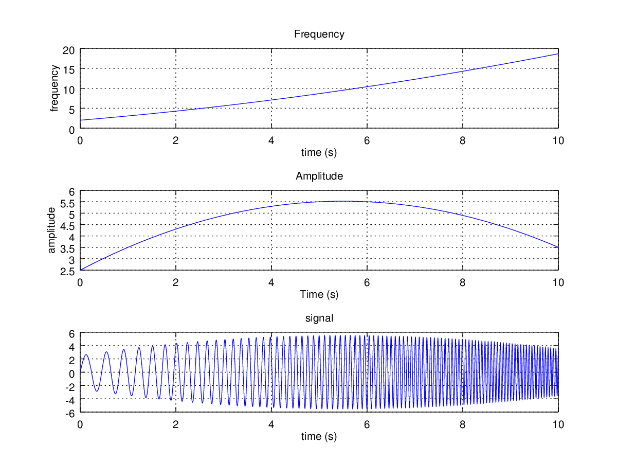
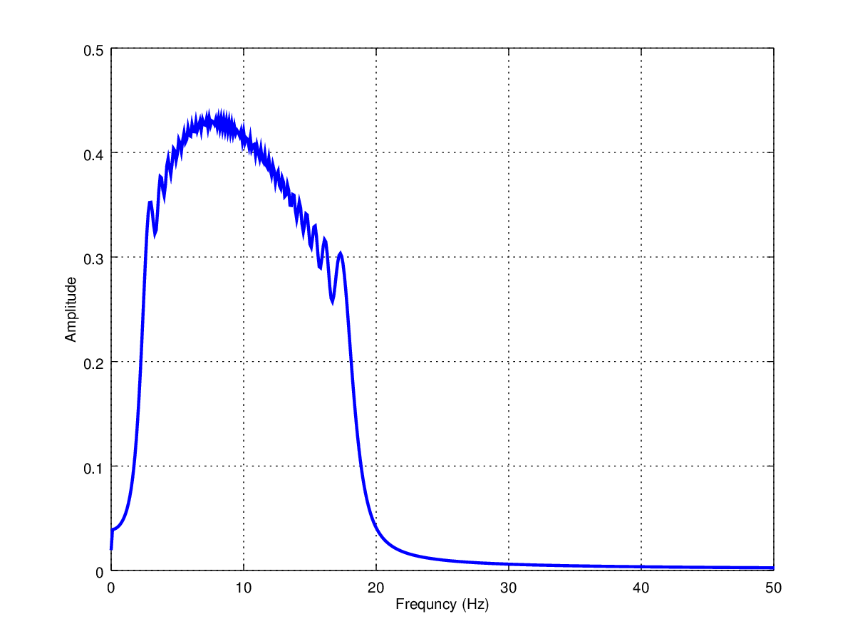
For a steady-state periodic vibration, say a motor running at a constant speed, the methods presented thus far are sufficient. But for transient (i.e. non-stationary) one is concerned with how the vibration changes with time. Taking an FFT of the entire time range will not be sufficient. To illustrate this, consider the example signal in Figure 28. Both the amplitude and frequency are changing as a function of time. As it is a simulated signal, we know the amplitude and frequency a priori. In the real world, we would have the signal from some measurement, and would be trying to figure out the amplitude and frequency content from the signal. A simple FFT of this signal is shown in Figure 29. The FFT tells us something about the signal, there is some frequency content that is spread out from about 0 to 20 Hz. But the FFT is telling us nothing about how the amplitude or frequency is varying with time.

Figure 28: Simulated signal to illustrate some time-frequency processing methods. The bottom plot shows the signal, the top two plots show the amplitude and frequency used to generate it.

Image stft_example_signal

Figure 29: An FFT applied to the signal in Figure 28

Image stft_example_motivation


Subsections
next up previous contents
Next: Short time Fourier transform Up: Vibration Data Analysis Previous: Impulsive noise   Contents " . $row['Name'] . " Posted on " . $row['DateTime']; echo "
"; echo $row['Comment']; echo "

"; } echo "
"; ?> Leave a comment on this page:

Name: (optional)
To prove you are not a robot, what is 2+3?

Creative Commons License
This work by Daniel Kiracofe (daniel dot kiracofe at gmail dot com) is licensed under a Creative Commons Attribution-NonCommercial-ShareAlike 4.0 International License./' $I