This method is straightforward. Imagine that you have an encoder (or perhaps a toothed wheel with a hall-effect pickup) on the rotating shaft in question which will give you a pulse for every 6 degrees of rotation (e.g. 60 pulses per revolution). Then, setup your data acquistion system to record one sample every time a pulse is received. So, if there was some vibration that happened once per rev, we would see a peak every 60 samples, regardless of the shaft speed. Similarly, a 2/rev vibration would show a peak every 30 samples. It would then be a simple matter to bandpass filter the signal to recover the 1/rev, 2/rev, etc. components. Such a filter would have a constant order bandwith. For example, if you created a bandpass filter between 0.9/rev and 1.1/rev, then at 600 RPM it would be equivalent to filtering between 9 Hz and 11 Hz, but when the shaft spins up to 1200 RPM, it is equivalent to filtering between 18 Hz and 22 Hz. The former is a 2 Hz passband width and the later is a 4 Hz passband width, but both represent 0.2 order bandwidth.
More than likely, however, you do not have such a setup and have sampled your signal the normal way at a constant time rate. It is a simple matter, however, to resample the signal. That is, using interpolation to determine what the value of the signal would have been at points that are spread out evenly in the angular domain. Matlab's interp1() command will do this.
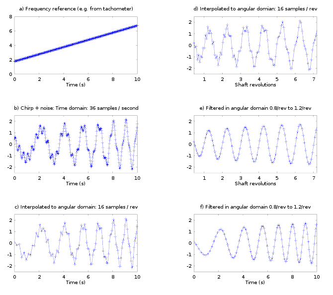
The process is illustrated in Figure 33. In (a) we have plot of frequency versus time. In (b) we have a signal with one component at the frequency in (a) as well as a constant higher frequency noise on top. This signal is evenly sampled in the time domain at 36 samples/second. We wish to remove the constant frequency noise and retain only the chirp. Since we know the frequency versus time, we can interpolate and resample the signal to be evenly spaced in the angular domain (c). Here we have 16 samples per revolution. In (d), we plot the same signal, but versus shaft angle instead of versus time. Note the signal that was increasing in frequency when plotted versus time is constant frequency when plotted versus shaft revolutions. Now it is a simple matter to just bandpass filter (e.g. in matlab we could use [b,a] = butter(2, [0.8, 1.2] / (Samples_per_rev/2) )). The result in (e) shows that the noise has been completely removed. Converting back to the time domain, we recover the original chirp signal (f).
Steps e and f in the figure are not necessary for order tracking, just for illustration. In practice, once you have the signal sampled in the angular domain, you can directly compute the order magnitudes. If you want all of the orders, take an FFT of the signal. Interpreting the signal as sampled at N samples/rev, the FFT amplitude in bin N is the 1st order, the amplitude at bin 2N is the 2nd order, etc. If you just want one single order, an FFT is too computationally expensive. Instead, use the https://en.wikipedia.org/wiki/Goertzel_algorithmGoertzel algorithm.
The biggest potential pitfall is aliasing. For example, maybe you have a shaft which has a gear on it with 40 teeth. The gear will produce a vibration signal at 40/rev. If you resample to, say, 12 samples/rev, you cannot represent the gear vibration signal per Nyquist's theorem and it will be aliased. In order to avoid this, you must either filter out higher frequency components first, or make sure you take enough samples/rev to capture all of the relevant orders. This can get more complicated if you have some vibration signals which are constant frequency. For example, many aircraft have AC power at a constant 400 Hz. If your shaft is running at 1000 RPM, then AC power is at the 24th order of the shaft, so you need to take 48 samples/rev to avoid aliasing. But if your shaft spins down to 500 RPM, then you need 96 samples/s to avoid aliasing.
There can also be some artifacts introduced by resampling. The resampling process can never recreate the true angular domain signal, only an approximation to it. These artifacts can be mostly supressed by choice of appropriate interpolate technique. For example, a cubic spline interpolation is much better than a linear interpolation (at the expense of more processing time). Higher sampling rates in the time domain also help.