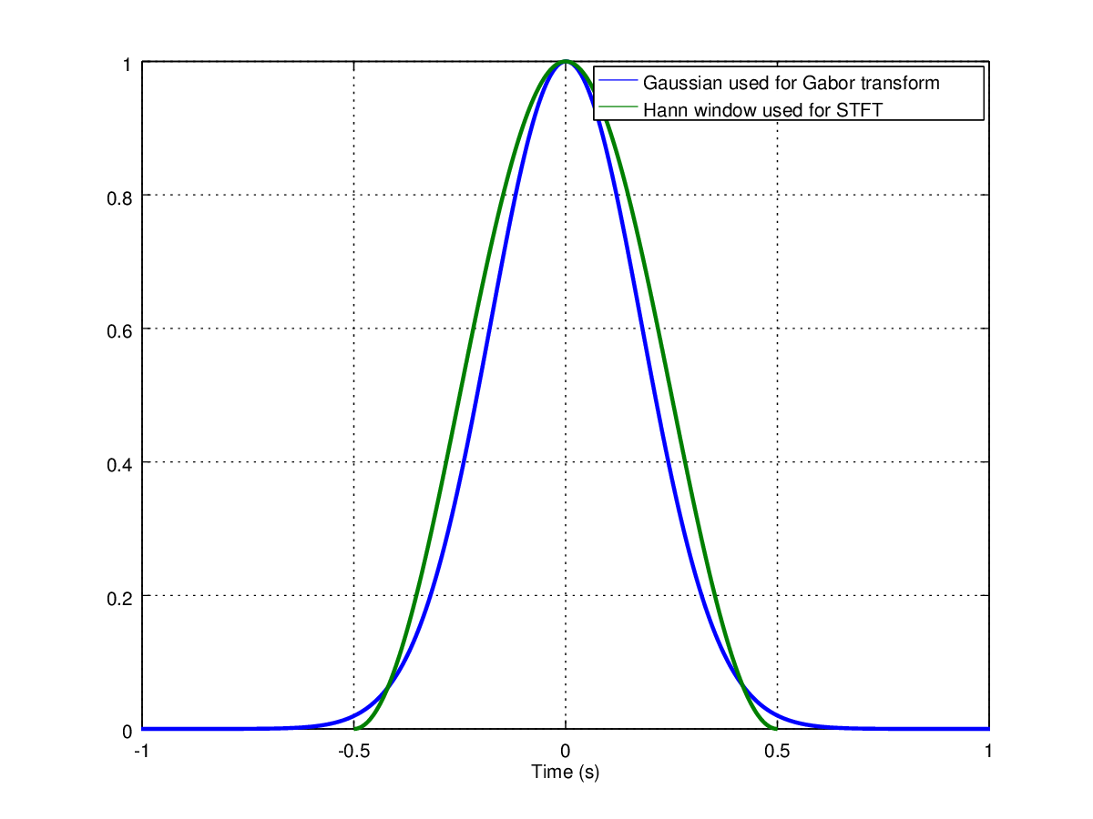
The Gabor transform is very similar to the STFT except the window function is replaced by a Gaussian (i.e. the normal distribution). A key characteristic of a window function (e.g. the hann window) is that it is exactly zero outside a specified range. However, a Gaussian asymptotically approaches zero but does not ever actually reach zero (see Fig 32). Mathemetically, this means that the Gabor transform has some nice properties. For example, the Gabor transform is invertible. You can recover the original time domain signal from the Gabor coefficients, but you cannot do that with a general STFT (http://zone.ni.com/reference/en-XX/help/372416A-01/svtconcepts/oa_methods/).
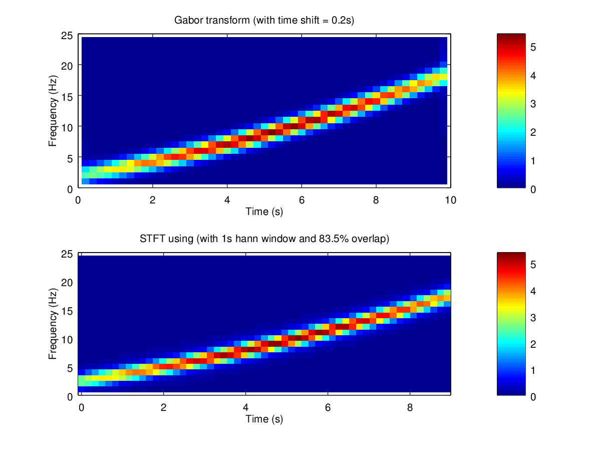
However, for many practical purposes there is not that much difference between using a STFT with a finite window and using the Gabor transform, assuming that approximately the same width window is used. See Figure 31.
Some nice codes to compute Gabor transforms are included in the Large Time-Frequency Analysis Toolbox (http://ltfat.sourceforge.net/). Note that the LTFAT function to compute a Gabor transform (dgtreal) has a similar issue as matlab's fft(). You have to scale the resulting coefficients by the sum of the window function to get back to engineering units. The code below was used to generate Figure 31.
%compute Gabor transform
M = Fs; % number of freq bins * 2 for Gabor transform
a = 200  % time shift in samples
[c, Ls, gw]=dgtreal(signal,'gauss',a,M); % c is the complex Gabor coefficients.  gw is the actual Gaussian window used
cc = abs(c) / (sum(gw)/2); % scale for the norm of the window function.
|