IIR filters (aka recursive filter) are typically designed by designing an analog filter and then converting to an equivalent digital filter. This typically works well, with some exceptions. For example, if the cutoff frequency is nearly half the sampling frequency or nearly zero, the filter behavior is usually less than ideal.
Figure 3 shows the problems that can arise with cutoff frequencies very close to the Nyquist frequency. The digital filter deviates significantly from its analog counterpart. This an inherent limitation of the process that is used to convert the analog filter to digital. If you are in this situation, the suggestion is to either design a digital filter directly (instead of converting an analog prototype) or increase the sampling rate.
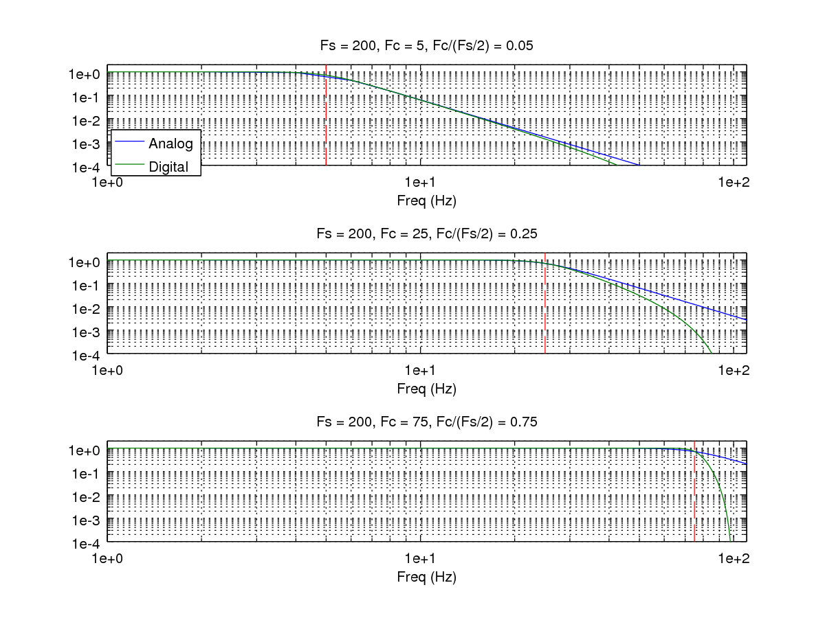
Figure 4 shows the problems that can arise with cutoff frequencies very close to zero (relative to the sampling rate). For very small cutoff frequencies, the filter becomes numerically unstable.
For those interested in the details of exactly why the low frequency problems happens, we need to understand round-off errors in float point arithmetic. The numerical precision of a floating point operation is usually characterized by the value epsilon, which is roughly defined as the maximum roundoff error when rounding down to 1. This value is stored by matlab in the pre-defined variable eps. For my machine, eps= 2.2204e-16. To see this in action type (1+1e-16)-1 at your matlab prompt. Clearly, the answer should be 1e-16, but my machine returns 0. For another example, try (1+3e-16)-1. The answer should be 3e-16, but matlab returns 2.2204e-16. So basically, if two numbers differ by more than about 16 orders of magnitude, we cannot compute the addition correctly.
With that in mind, let us examination the filter coefficients generated by [b,a] = butter(2, fc/(Fs/2)) in Table 1. Recall that the basic form of a filter is a(1)*y(n) = b(1)*x(n) + b(2)*x(n-1) + ... + b(nb+1)*x(n-nb) - a(2)*y(n-1) - ... - a(na+1)*y(n-na). In this example, the inputs x are on the order of 1, the outputs y are on the order of 1, and the coefficients a are on the order of 1 - 10. So for the cutoff frequency 0.0002, the worst case would be that we add a value of about 6 to a value of about 9e-15. Try (6+9e-15)-6 at your matlab prompt. I get 8.88e-15. Pretty close, but there is some roundoff error. Now look at cutoff frequency 0.0001. Now we need to try (6+6e-16)-6. I get 8.88e-16. Relative to the expected answer, that's a pretty big error. Since the IIR filter uses feedback, errors like this get fed back into the computation and cause the problems seen in the graph.
If you ever find yourself in this type of situation where you must use a very low cutoff frequency, the best option is to decimate your data. In other words, downsample it to a lower frequency first. That way, the same physical cutoff frequency is a much larger percentage of the sampling frequency and the calculations can proceed. Another option would be to use a lower order IIR filter, or to use an FIR filter.
|
![\includegraphics[bb=0bp 195bp 612bp 600bp,clip]{butter_low_freq}](img5.png)
|
|
There are other design methods for IIR filters that do not involve starting with an analog prototype. See, for example, the yulewalk function in Matlab [9].
