The so-called enveloped FFT (sometimes called the acceleration enveloped FFT because it is most commonly used on accelerometer data) is a technique for analyzing repetitive impacts. The canonical example is a defect on a rolling element bearing, but it might also be aplicable to other situtations - gear tooth defects perhaps. Bentley Nevada has a good application note on this[5]. I will give a very short summary here.
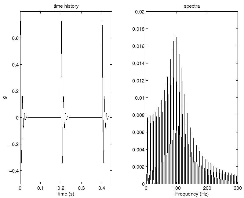
Take as an example a ball bearing where there is a defect on one race such that a ball passes this defect at a rate of 5 Hz. Further, assume that the bearing housing has a natural frequency of 100 Hz. Every time the ball passes the defect, the impact will ring the natural frequency of the housing - a series of small pings. This is shown in 22. The time history is fairly easy to interpret since this one simulated defect is the only signal present. In a real situation, there will be many other effects (shaft unbalance, other bearing frequencies, etc.). When the situation gets complicated, we might like to turn to a frequency domain representation, and pull out the component corresponding to the defect frequency. We could then trend on this component over time to see if the defect is getting worse. But look at the spectrum in this figure. It is not going to be easy to interpret. There is energy at 5 Hz and 100 Hz, but also at many other frequencies. The dominant component is at 100 Hz, not 5 Hz. This will not be easy to trend on.
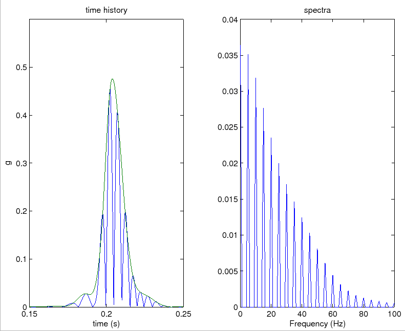
The enveloping process is as follows: first we band pass filter around 100 Hz to remove noise. Then we rectify the signal (take absolute value), and find the envelope (see 5.3). Then the spectrum of the enveloped signal is found. Now the strongest component is at the defect frequency (and a few harmonics). Effectively, we have taken energy which was spread out over the spectrum and moved it down to the defect frequency. Now it will be easier to trend upon this component and see if it increases with time.
|